QCORE Seminar Series · November 5, 2025
Featuring Brian D’Urso
📄 Access the full slide deck
Why We Hosted This Talk
At QCORE, we highlight research that sits at the intersection of fundamental science and real-world technological capability. Some of the most important questions in quantum science aren’t only about building new devices—they’re about understanding the limits of measurement itself.
How precisely can we detect motion?
What sets the boundary between classical sensing and quantum-limited sensing?
And how do real experimental systems approach those limits?
In this seminar, Brian D’Urso walked us through the physics of position detection in levitated optomechanics, showing how researchers can trap microscopic objects in ultra-high vacuum and measure their motion with extraordinary precision—sometimes at scales far smaller than a single atom.
The talk offered a practical, hands-on look at the measurement problem: not just the theory, but the experimental reality of photons, momentum transfer, shot noise, and the surprising ways these effects can be exploited rather than avoided.
About the Speakers
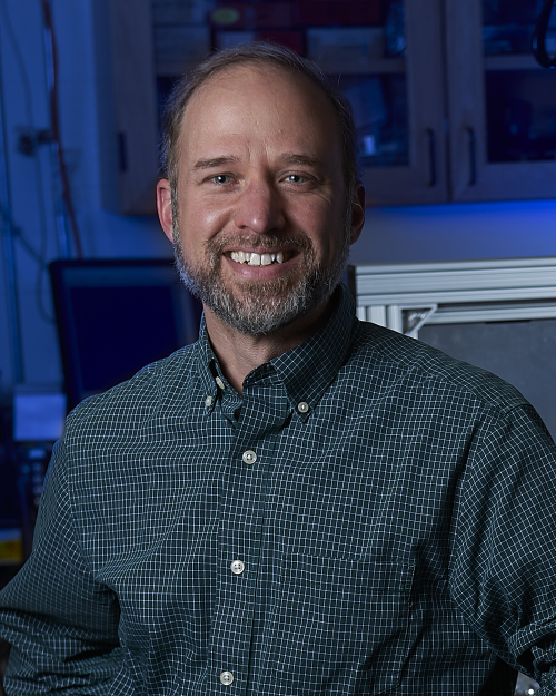
Professor Brian D’Urso
Brian D’Urso is a physicist whose research explores levitated optomechanics, quantum-limited measurement, and precision sensing. His lab develops experimental systems that trap small objects—often micron-scale particles—using magnetic fields, and then measures their motion using optical detection techniques in ultra-high vacuum environments.
His work sits at the crossroads of quantum measurement theory and experimental instrumentation, where the challenge is not simply observing a system, but understanding how the act of measurement itself shapes what can be known.
Opening: Microfabrication Trauma and a Warning About Dropping Chips
Brian begins with a light memory from his undergraduate days learning microfabrication. He jokes that there are countless ways fabrication can go wrong, but the most painful is a scenario many researchers can relate to:
You spend days making a chip, you’re almost finished… and then you drop it.
And suddenly you’re on the floor, searching under equipment in the dirt, trying to recover the fragile object you just spent days building.
It’s funny—but it sets the tone. This is a talk grounded in experimental reality.
Then he tells the audience he’s going to structure the talk in an unusual way: he will spend the entire seminar convincing us of one point… and then explain why that point is wrong.
That’s the framework.
What Is Levitated Optomechanics?
Brian explains that levitated optomechanics is the study of trapping small objects—often particles ranging from microns to millimeters—and using light (or fields) to measure and control their motion.
In its simplest form, it’s the physics of taking something small and levitating it, then watching what it does.
He describes three common trapping approaches:
- Optical traps, where a focused laser beam holds an object in place
- Paul traps, which use alternating electric fields (electrodynamic ion trapping)
- Magnetic trapping, specifically diamagnetic trapping, which is the approach used in his lab
He notes that diamagnetic trapping has famously been used to levitate frogs, but in his lab they focus on smaller objects—particles from micron to millimeter scale.
Why Vacuum Matters
Brian emphasizes that the key to making levitated systems scientifically useful is vacuum.
They work in vacuum because air molecules collide with the trapped particle and push it around so strongly that the particle’s motion becomes dominated by gas interactions. In that case, the experiment doesn’t measure the physics of the trapped object—it measures the physics of air.
Instead, they work in ultra-high vacuum: on the order of 10⁻¹⁰ torr, which he describes as roughly 10⁻¹³ atmospheres.
At that pressure, the particle becomes isolated enough that subtle forces become visible.
How the Magnetic Trap Works
Brian then explains the physical construction of the trap, and he emphasizes how deceptively simple it looks.
The trap consists of two permanent magnets (he jokes they’re only “a little stronger than refrigerator magnets”), surrounded by four pole pieces that shape the magnetic field.
The pole pieces can be iron, though his lab uses a stronger alloy called Hyperco 50, which improves the field strength.
The levitated particle sits in a gap between the magnets that is only about a quarter of a millimeter wide.
That tiny gap is crucial. The levitating force depends on the gradient of the magnetic field squared—essentially the gradient of B²—so the field must be strong and the gradient must be sharp.
And that’s why he jokes he can’t levitate a person: the physics works, but humans don’t fit in a quarter-millimeter gap.
Seeing the Particle: The Optical Measurement System
After describing the trap, Brian shows what the experiment looks like in practice.
A particle is levitated inside ultra-high vacuum, and a set of optical components surround the trap. The job of these optics is straightforward:
Measure the position of the levitated object by scattering light off it.
He shows an image of a bright dot—about a 1 to 1.5 micron silica sphere—floating in vacuum.
The particle is not directly “seen” like a normal object. Instead, it is detected through how it scatters light.
The optics system is designed to translate scattered light into a precise estimate of the particle’s motion.
What the Data Looks Like: A Noise Spectrum of Motion
Brian then introduces the type of data his lab collects.
He shows a frequency-domain spectrum: frequency on the horizontal axis (log scale), and displacement noise on the vertical axis.
The plot contains three curves corresponding to three different optical power levels.
At high frequencies, something important happens:
As optical power increases, the measured noise decreases.
That makes intuitive sense: more photons give more measurement information.
But Brian points out that the story is more complicated, because not all noise is measurement noise.
He explains that the low-frequency region contains resonances because the trapped particle behaves like a harmonic oscillator. In the mid-frequency region, the spectrum is dominated by thermal effects.
The part he cares about most is the high-frequency region, where noise is flat and power-dependent.
The Three Major Noise Sources
To explain the shape of the spectrum, Brian introduces the three main sources of noise in the experiment.
1. Thermal Noise
This is classical and relatively straightforward. Even at 10⁻¹⁰ torr, residual gas molecules collide with the particle and push it around. Thermal noise typically has a spectrum that scales like 1/f².
2. Radiation Pressure Shot Noise (Back Action)
This is more subtle and starts to touch quantum behavior. Photons carry momentum. When photons scatter off the particle, they act like tiny billiard balls. Each photon gives the particle a random push.
The pushes are random because photon arrivals follow shot noise statistics. This produces back-action noise that also scales like 1/f², because the particle’s response falls off with frequency.
3. Detector Shot Noise (Measurement Noise)
This is the noise that dominates at high frequencies. Even if the particle is perfectly still, the detector receives photons in a random arrival distribution. That randomness produces uncertainty in the measured signal. This is the noise that decreases as optical power increases.
From Images to Motion: The Cross-Correlation Tracking Method
Brian then explains one of the most practically impressive parts of the experiment: converting raw camera images into position data.
The lab records video frames of the particle, then compares images to determine how much the particle moved between frames. Instead of tracking the particle with a simplistic centroid method, they use a statistically optimized approach:
They compute the cross-correlation between frames and perform a weighted minimization that accounts for shot noise in each pixel.
He explains that this is mathematically equivalent to a chi-squared minimization, and the key computational advantage is that cross-correlations can be done efficiently in the Fourier domain. This means the lab can run the analysis in real time using GPU computation.
The result is extremely precise position tracking—well below the pixel scale.
Picometer Precision: Measuring Motion Smaller Than an Atom
Brian then returns to the earlier spectrum and points out the magnitude of the best measurement performance.
At the highest power levels, the position noise is around 4 picometers / √Hz. With one second of averaging, they can locate the particle’s position to within about four picometers.
And yes—that is far smaller than the size of a single atom. He admits that this result can feel unsettling. How does it make sense to locate the position of an object that is a micron across to a precision far smaller than atomic dimensions?
He argues that the measurement is meaningful: the particle’s motion can still be tracked with extraordinary precision even if the particle itself is large.
The Central Claim: Two Ways to Derive the Same Measurement Limit
At this point, Brian arrives at the key point of the talk. He writes down an expression for detector shot noise. The expression shows that position uncertainty depends on:
- wavelength (λ)
- number of photons scattered (Nλ)
- a constant ε related to momentum transfer
He notes the familiar scaling. Position noise decreases as 1/√N. That’s expected from shot noise.
But the deeper idea is this: If we truly understand the measurement, we should be able to derive the same result from two different perspectives.
And he argues that there are two equivalent ways to think about position detection limits:
1) Momentum Transfer Perspective
Photons scatter off the particle. Their scattering angles determine how much momentum they transfer. If the momentum kicks are random, we can compute the resulting momentum noise.
Then, using the Heisenberg uncertainty principle, we can connect momentum uncertainty to position uncertainty.
2) Diffraction / Optical Resolution Perspective
From optics, we expect a diffraction-limited resolution of roughly:
λ / (2 NA)
And again the result scales as 1/√N.
So the two frameworks should match.
This is the point he spends the talk building toward.
Three Particle Cases: When the Simple Argument Works… and When It Doesn’t
Brian then tests his argument against three different experimental particle types.
Case 1: A Small Silica Sphere
For a micron-scale silica particle illuminated by a plane wave, the argument works cleanly.
You can compute the scattering pattern using Mie scattering. From the scattering distribution, you can compute the momentum transfer. From momentum transfer, you can compute expected measurement noise.
And you can also compute it optically by looking at the effective numerical aperture of collected light. These match nicely.
Case 2: An Opaque Graphite Particle
Brian then shows a larger particle: a dark graphite chunk. Now the situation becomes more complicated.
Most photons hit the graphite and get absorbed, transferring momentum but giving no information.
That’s acceptable because the uncertainty principle contains a ≥ sign. Lost photons add momentum noise but do not improve measurement precision.
So where does the measurement information come from? Brian argues it comes from the photons that graze the edge of the particle—photons that diffract around the boundary.
Those photons carry the positional information, because they encode diffraction effects that can be detected.
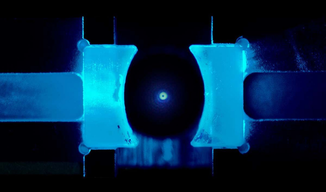
Case 3: A Transparent Glass Sphere (The Weird One)
The most interesting case is a transparent glass sphere. Brian shows a ~60 micron borosilicate glass sphere that appears dark in the image even though it is transparent.
The explanation is that light is being deflected. Some photons travel around the sphere, producing edge diffraction that contains position information.
But photons that travel through the sphere do something else entirely: The sphere acts as a lens. It focuses the light into a bright spot in the center of the image.
This creates a multi-plane optical system where information exists in different focal regions. The diffracted photons and focused photons do not reside in the same plane, and collecting both optimally becomes difficult.
This is not simply an optical nuisance—it becomes a fundamental limitation on how efficiently measurement information can be extracted.
Why This Matters: Optimizing Information Collection
Brian briefly mentions that within the QCORE project, his team is working on optimizing this measurement process.
The goal is to maximize position information by engineering how photons interact with the trapped object and how the scattered photons are collected.
He doesn’t go into details, but the implication is clear:
At high precision, measurement is not just about having more photons. It is about using them efficiently.
The Twist: The Argument Is Not Universally True
Then Brian delivers the promised reversal. He explains that the semi-classical picture—momentum transfer on one hand, diffraction limit on the other—is not universally correct. It depends on a hidden assumption in the uncertainty principle expression he’s been using.
The key assumption is:
Δx and Δp are uncorrelated.
But in the real experiment, the photons causing momentum kicks are the same photons being detected. That means the measurement noise and the back-action noise can become correlated. And if they are correlated, the “standard” uncertainty argument is incomplete.
Beating the Standard Limit: Canceling Shot Noise with Back Action
Brian explains that by deliberately manipulating the detection geometry—such as intentionally defocusing the detector or modifying the Gouy phase—one can create correlations between radiation pressure back-action noise, and detector shot noise. If tuned correctly, these can partially cancel.
This produces frequency ranges where the total measurement noise can drop below what the simple uncertainty argument would suggest.
He emphasizes this does not violate the uncertainty principle. Instead, it violates the assumptions behind the simplified inequality.
He notes that LIGO explored similar approaches in the past, and while modern LIGO uses squeezed light, the principle is related: measurement can be engineered to exploit quantum correlations.
A Deeper Question: What State Does the Particle End Up In?
Brian admits that when he thinks too deeply about this measurement process, it becomes conceptually confusing.
If you engineer a measurement that cancels noise, what happens to the quantum state of the particle? What does the measurement collapse into?
He doesn’t answer this in the talk—and explicitly says it’s a harder question than anything he covered. But it highlights the deeper philosophical and physical implications: at the quantum limit, measurement is no longer passive observation. It becomes a process that shapes reality.
Closing Acknowledgments
Brian credits his graduate students for the work, and thanks funding sources including the National Science Foundation and AFRL.
Q&A Highlights
Q1 — Is the bright spot in the glass sphere caused by interference?
A: Brian explains that the bright central spot is not primarily caused by interference or diffraction effects. It is caused by the transparent sphere acting as a lens and focusing the light. The spot is extremely bright and saturated compared to the rest of the image. He notes there may be some diffraction contribution, but the lensing effect dominates.
Q2 — What “position” are we actually measuring in a transparent object?
A: Brian suggests that what they measure is closer to an “optical center of mass,” not the gravitational center of mass. It’s an effective optical measurement quantity rather than a literal physical center.
Q3 — Could internal vibration modes of the object interfere with the measurement?
A: Brian says almost certainly the particle has internal vibration modes, but these modes are typically at much higher frequencies than what the experiment measures, especially for small particles. That separation in frequency makes the modes weakly coupled to the observed motion, which helps simplify the analysis. For larger particles, it could become more of a concern.
Q4 — Do students learn uncertainty analysis and systematic error tracking in this work?
A: Brian explains that uncertainty analysis depends on the type of project. In optomechanics papers, uncertainty accounting is not always emphasized. But in precision measurement work—such as his group’s efforts related to measuring the gravitational constant G—students must rigorously track statistical and systematic uncertainties, often reporting them in structured tables. He notes that uncertainty analysis is also practiced in advanced undergraduate and graduate physics labs.
Q5 — Does gravity affect the trap?
A: Brian explains that Earth’s gravity significantly displaces the particle downward, and the trap design actually relies on Earth’s gravity to keep the particle stable. In fact, he notes that if the same trap were taken into outer space, the particle might escape due to symmetry effects in the trapping configuration. He adds that gravitational attraction between two trapped particles would be extremely small, but Earth’s gravitational field is dominant.
| Ask Brian Have a question about levitated optomechanics, quantum-limited measurement, or how light can be used to detect motion with picometer precision? Send it our way—Brian may answer it in an upcoming QCORE feature. ➜ Submit a question |